This configuration will require an additional piece of equipment, a second red pitaya. One red pitaya will be used as in the oscilloscope/signal generator or the spectrum analyzer modes, while the other will be used in the LTI DSP workbench. Connect the red pitayas such that the IN1 of the LTI DSP device is connected to OUT1 of the generator. You can also use a T-joint to connect the OUT1 of the generator board to IN1 of itself to see the response of the circuits more clearly and to measure the Frequency response with the Bode analyzer.
Running Sum Filter
This is a classical FIR filter that operates with the following difference equation
This has the z domain transfer function of simply the sum each delay element multiplied by unity.
Where the final transfer function expression is simply the expansion of the M-th partial sum of a geometric series for |z|<1.
MATLAB Analysis
- In the provided matlab script, vary the number of taps (value of M) for the running sum filter and comment on as to how the:
- Impulse response changes
As the number of taps increases, the impulse response becomes longer, capturing a larger portion of the input history.
b. Frequency response changes
Increasing the number of taps allows for sharper frequency cutoffs and improved stopband attenuation.
c. Pole zero plot behaves
The pole-zero plot will show M zeros at the origin.
- If we assign all , this is the moving average filter from the previous lab, how does this valuing of the values change:
- Impulse response
The impulse response will have a flat top and a gradual decay.
b. Frequency response
The frequency response will have a flat magnitude response in the passband and roll-off in the stopband.
c. Pole zero plot
The pole-zero plot will show M zeros at the origin.
Red Pitaya
In the red pitaya’s LTI workbench, we can construct arbitrary transfer functions using the coefficients where k∈[0,5] with the caveat that =1. Expanding the transfer function of the running sum filter to accommodate this maximal number of taps yields the following transfer function
This shows that all values are 1, and that =1.
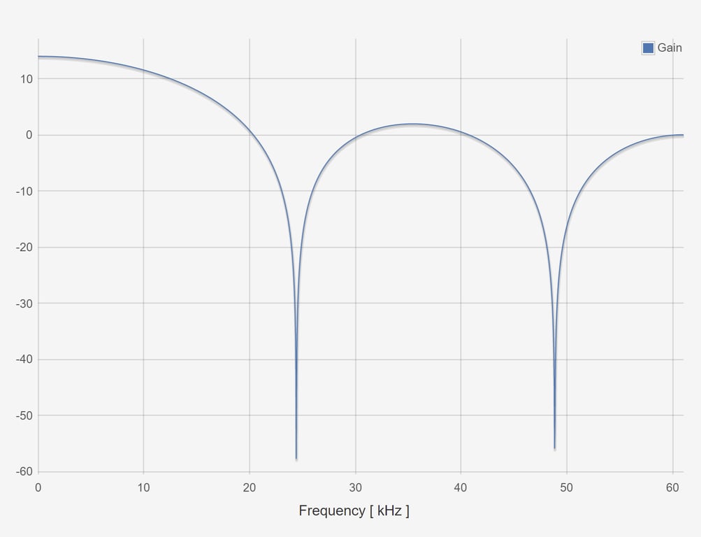
- Plot the frequency response of this filter when entered into the red pitaya LTI workbench.
- Show to resulting filtered waveforms/spectra to a:
- Square wave within the filter bandwidth
b. Square wave outside of the filter bandwidth
 Made with Bullet