This configuration will require an additional piece of equipment, a second red pitaya. One red pitaya will be used as in the oscilloscope/signal generator or the spectrum analyzer modes, while the other will be used in the LTI DSP workbench. Connect the red pitayas such that the IN1 of the LTI DSP device is connected to OUT1 of the generator. You can also use a T-joint to connect the OUT1 of the generator board to IN1 of itself to see the response of the circuits more clearly and to measure the Frequency response with the Bode analyzer.
Resonant Filter
This is a classical IIR filter that operates with the following difference equation
Which describes a feedforward of the input with a delayed version of the output. Intuitively, for periodic signals, this implies that the filter will, when supplied a signal with fundamental period N will have reinforcing effect, whereby each of the previous peaks of a signal will be summed with the current peak of the signal to provide large gain at this specific frequency. This behavior is known as resonance, and is commonly used to design many kinds of filters. Mapping this to the z-domain provides the following equation:
Which after some algebra, provides the transfer function of:
MATLAB Analysis
1. In the provided matlab script, vary the feedback delay (value of N) for the resonant filter and comment on as to how the:
a. Impulse response changes
The impulse response will exhibit resonance at the frequency determined by the feedback delay.
b. Frequency response changes
The frequency response will show a peak at the resonant frequency and roll-off in neighboring frequencies.
c. Pole zero plot changes
The pole-zero plot will show a single pole at z=1/N.
Red Pitaya
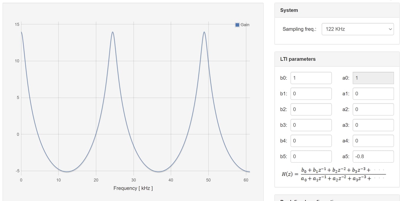
In the red pitaya’s LTI workbench, we can construct arbitrary transfer functions using the coefficients where k∈[0,5] with the caveat that =1. Expanding the transfer function of the resonant filter to accommodate this maximal number of taps yields the following transfer function
This shows that =1, =0 ∀ k∈{[1,5]∩ }, and that and =0 ∀ k∈{[1,5]∩ }.
- Plot the frequency response of this filter when entered into the red pitaya LTI workbench.
- Show to resulting filtered waveforms/spectra to a:
a. Square wave within the filter resonance. Step Response of the filter outside of the resonance
b. Step Response of the filter outside of the resonance
Filter Cascade
As mentioned previously, cascading two filters is described simply by multiplying their transfer functions.
Perform analysis on the resulting cascaded filter where are the running sum filter with 6 taps (M=6), and the resonant filter with order 6 (N=5).
MATLAB Analysis
Using the previous two filter transfer function in MATLAB, calculate the result of cascading the filters.
- Calculate the result of cascading the filters.
- Write out the resulting transfer function
- Plot and comment on the:
- Impulse response shape w.r.t either of the before filters
- Frequency response w.r.t either of the before filters
- Pole zero plot w.r.t either of the before filters
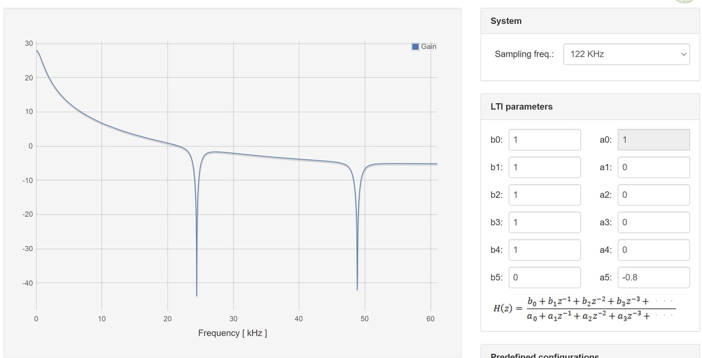
Red Pitaya
Enter the previously calculated transfer function into the Red Pitaya.
- Plot the frequency response of this filter
- Show to resulting filtered waveforms/spectra to a square wave at:
- Square wave within the filter bandwidth
b. Square wave outside of the filter bandwidth
 Made with Bullet